How To Hide Rows And Columns In Google Sheets

Hiding Rows in Google Sheets

If you're working with large datasets in Google Sheets, you may find that some rows or columns are not relevant to your current task or view. Hiding these unnecessary rows and columns can help declutter your spreadsheet and make it easier to focus on the data that matters. In this article, we'll show you how to hide rows and columns in Google Sheets, making it easier to organize and analyze your data.

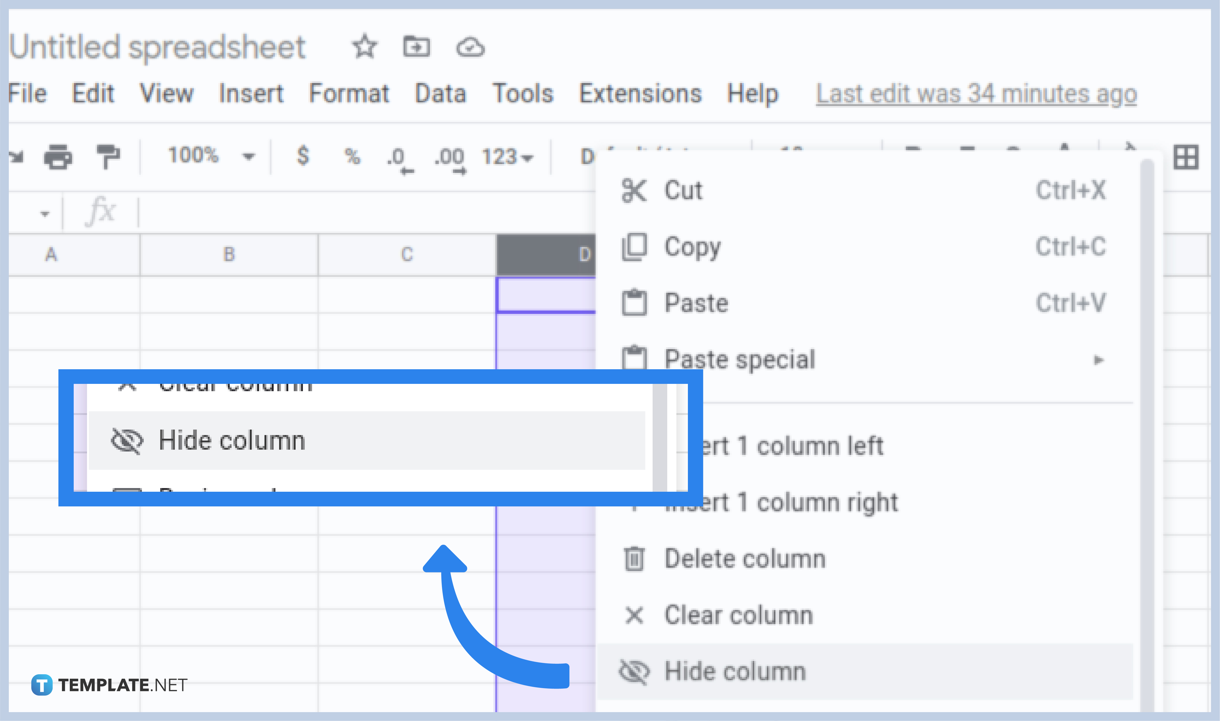
To get started, select the row or column you want to hide by clicking on the row or column header. You can also select multiple rows or columns by holding down the Ctrl key (or Command key on a Mac) and clicking on each row or column header. Once you've selected the rows or columns, right-click on the selection and choose 'Hide rows' or 'Hide columns' from the context menu.

Hiding Columns in Google Sheets

Hiding rows in Google Sheets is a straightforward process. Simply select the row you want to hide, right-click on it, and choose 'Hide row'. You can also use the keyboard shortcut Ctrl+Alt+0 (or Command+Option+0 on a Mac) to hide the selected row. If you want to hide multiple rows, select them all and use the same method. The hidden rows will be removed from view, but the data will still be preserved.

Hiding columns in Google Sheets is just as easy. Select the column you want to hide, right-click on it, and choose 'Hide column'. You can also use the keyboard shortcut Ctrl+Alt+0 (or Command+Option+0 on a Mac) to hide the selected column. If you want to hide multiple columns, select them all and use the same method. The hidden columns will be removed from view, but the data will still be preserved. By hiding rows and columns in Google Sheets, you can create a more organized and readable spreadsheet that helps you focus on the data that matters.